European Option Pricing

We price European call options under geometric Brownian motion

$$dS = rS\,dt + \sigma S\,dZ,$$

with parameters $S_0 = 100$, $K = 99$, $\sigma = 0.2$, $r = 0.06$, $T = 1$.

The GBM admits the closed-form solution

$$S_T = S_0 \exp\!\left[\left(r - \tfrac{1}{2}\sigma^2\right)T + \sigma\sqrt{T}\,Z\right],$$

which we discretise over $n$ time steps as

$$S_{t+1} = S_t \exp\!\left[\left(r - \tfrac{1}{2}\sigma^2\right)\Delta t + \sigma\sqrt{\Delta t}\,\phi\right], \quad \phi \sim \mathcal{N}(0,1).$$

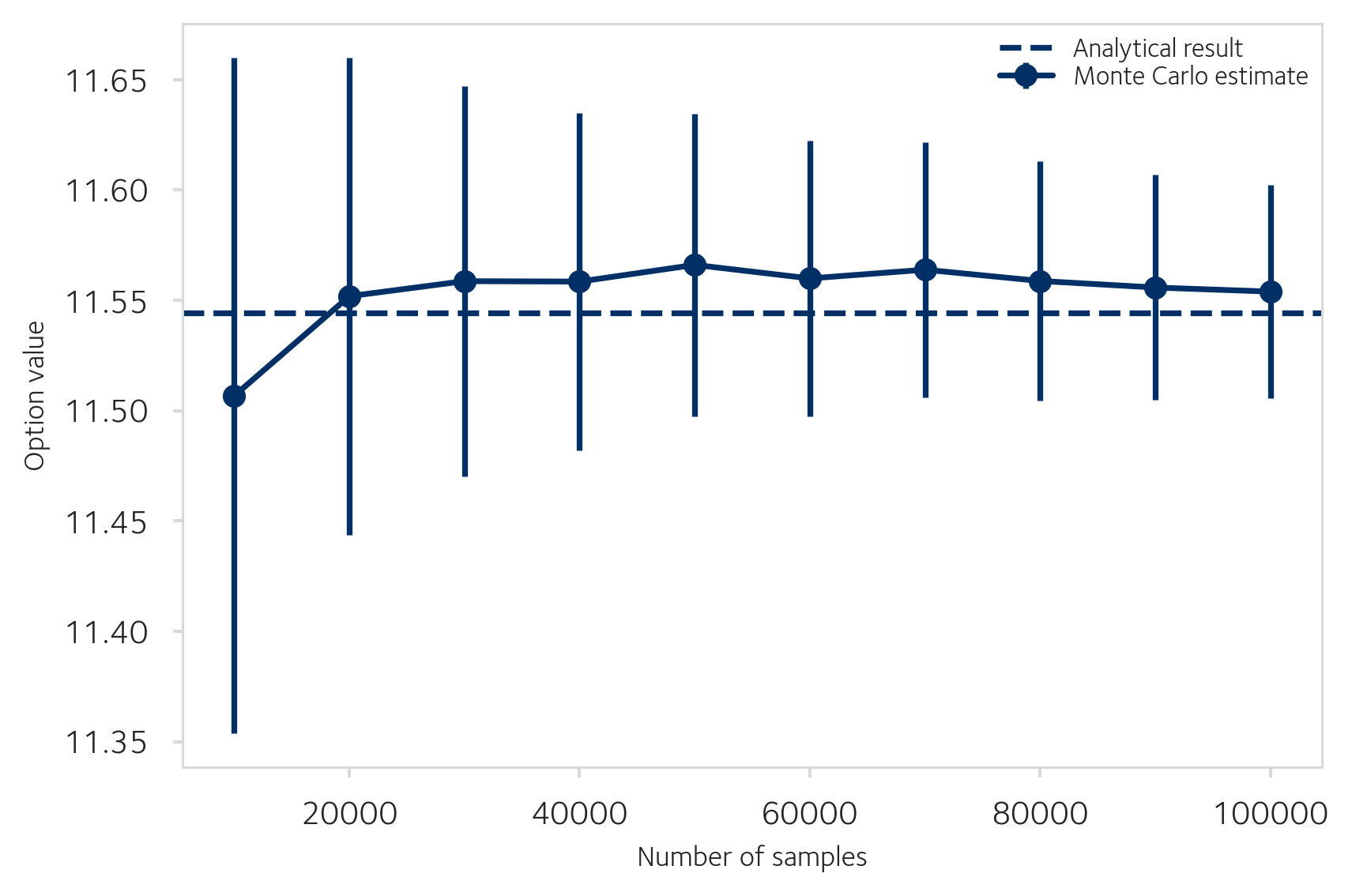
The discounted expected payoff $e^{-rT}\,\mathbb{E}[\max(S_T - K, 0)]$ is estimated by averaging over simulated paths. The Black-Scholes analytical price for these parameters is $V = 11.5443$ with delta $\Delta = 0.6737$.

Convergence

Increasing the number of Monte Carlo paths reduces the standard error as $\mathcal{O}(1/\sqrt{n})$.

Antithetic Variates

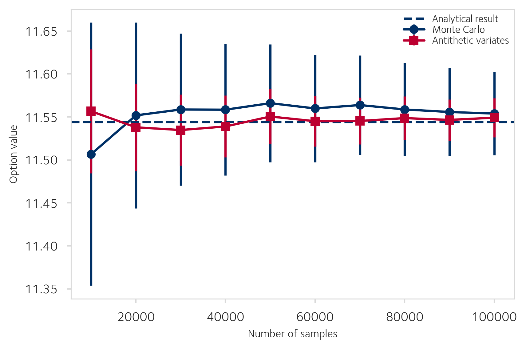
For each random draw $Z$, we also evaluate the payoff at $-Z$. Since the two payoffs are negatively correlated, their average has lower variance:

$$\hat{V} = \frac{1}{2}\left[f(Z) + f(-Z)\right].$$

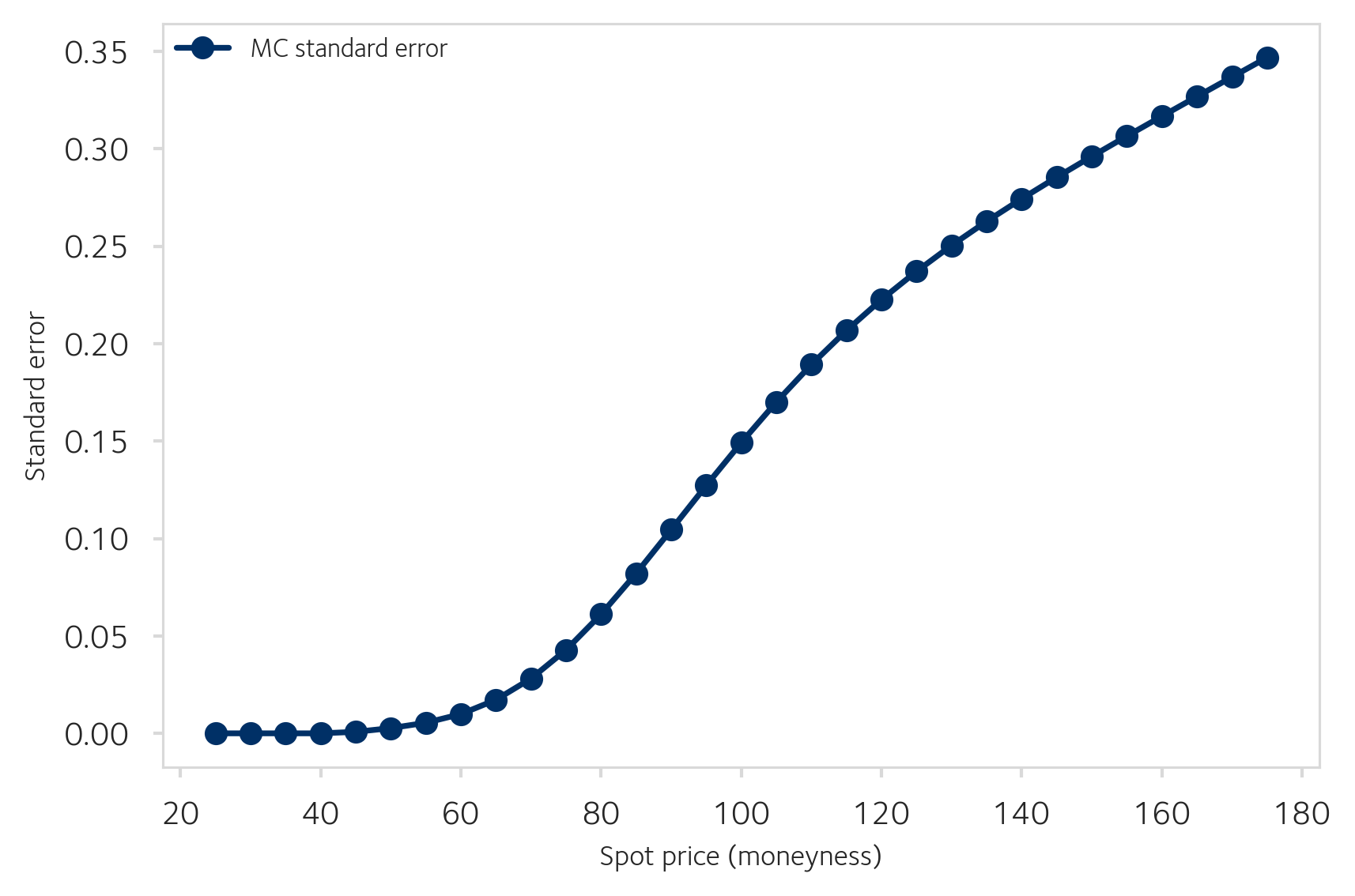
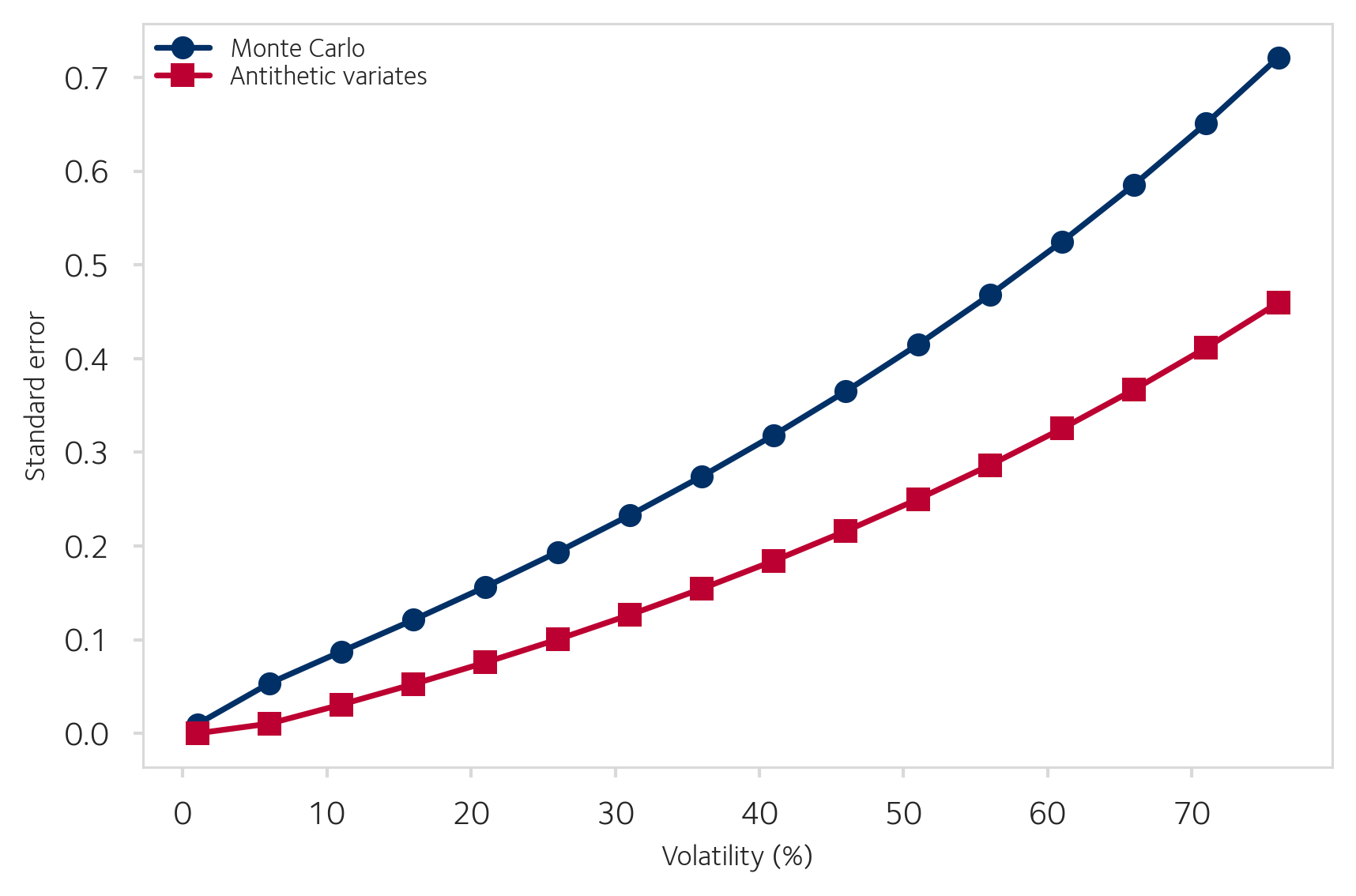
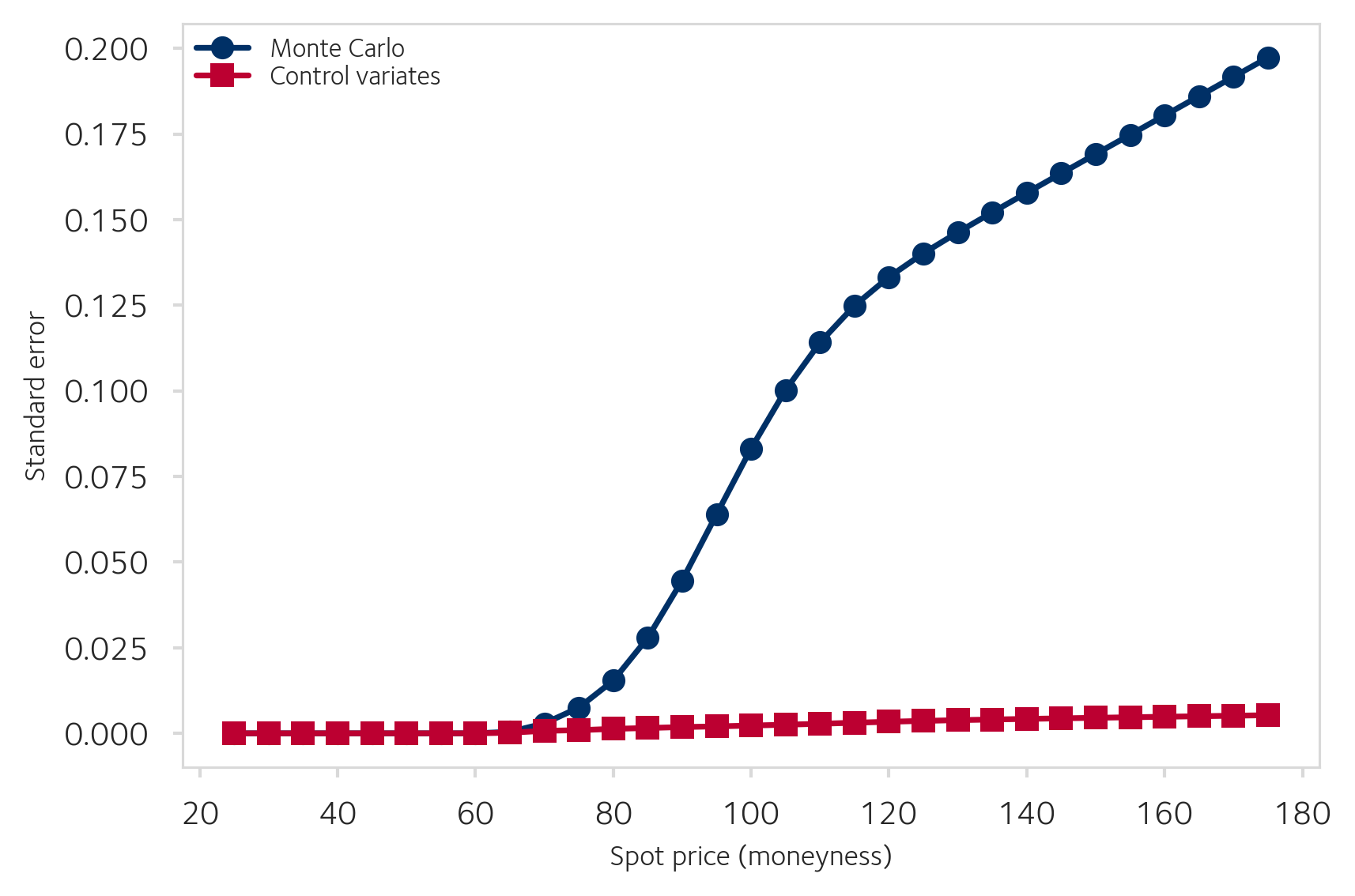
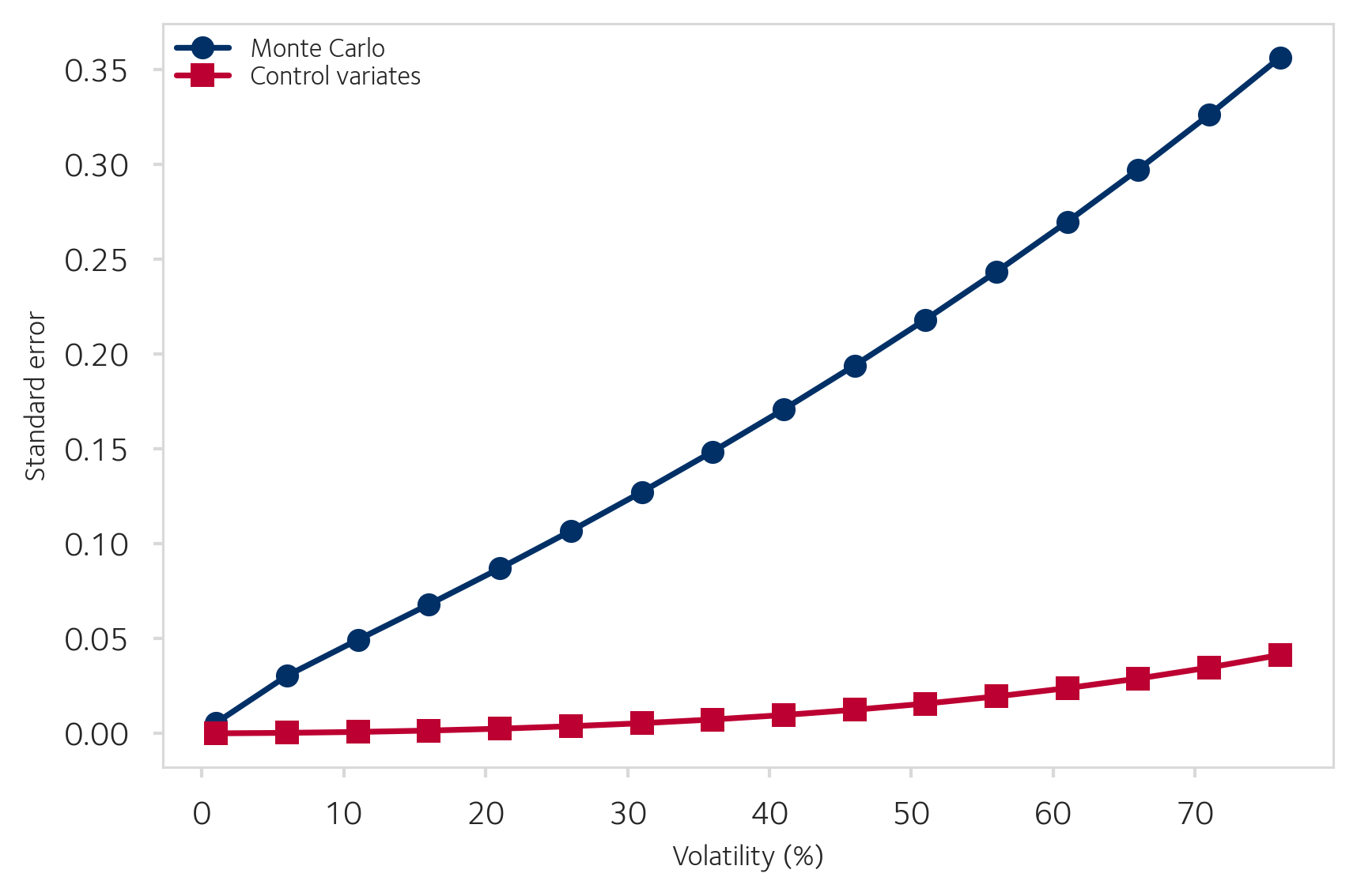
Standard Error vs Moneyness and Volatility

The standard error depends on the option’s moneyness and on volatility. Deep in-the-money options have less payoff variance; higher volatility increases it.

Sensitivity Estimation

The hedge parameter $\Delta = \partial V / \partial S$ is estimated by the bump-and-revalue method:

$$\hat{\Delta} = \frac{V(S_0 + \varepsilon) - V(S_0)}{\varepsilon}.$$

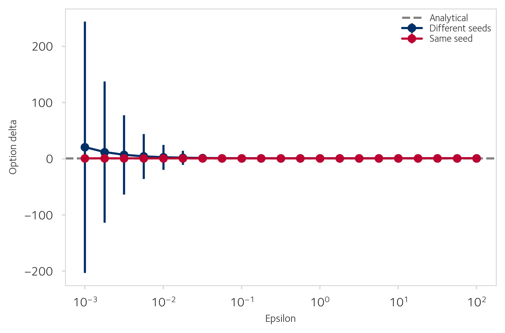
Seed Control

When different random seeds are used for the base and bumped simulations, the noise in each estimate is independent, and the finite-difference ratio becomes dominated by MC noise at small $\varepsilon$. Using the same seed ensures the same random draws, so the noise cancels in the numerator.

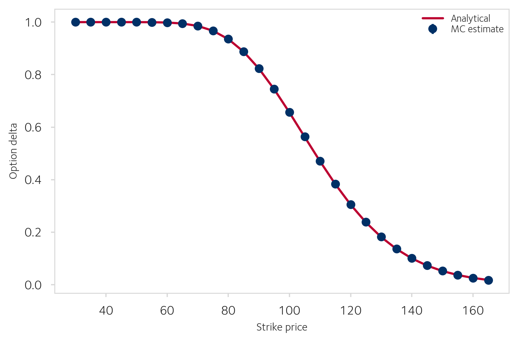
European Delta vs Strike

With the same-seed approach, the MC delta estimate tracks the analytical Black-Scholes delta across the full range of strikes.

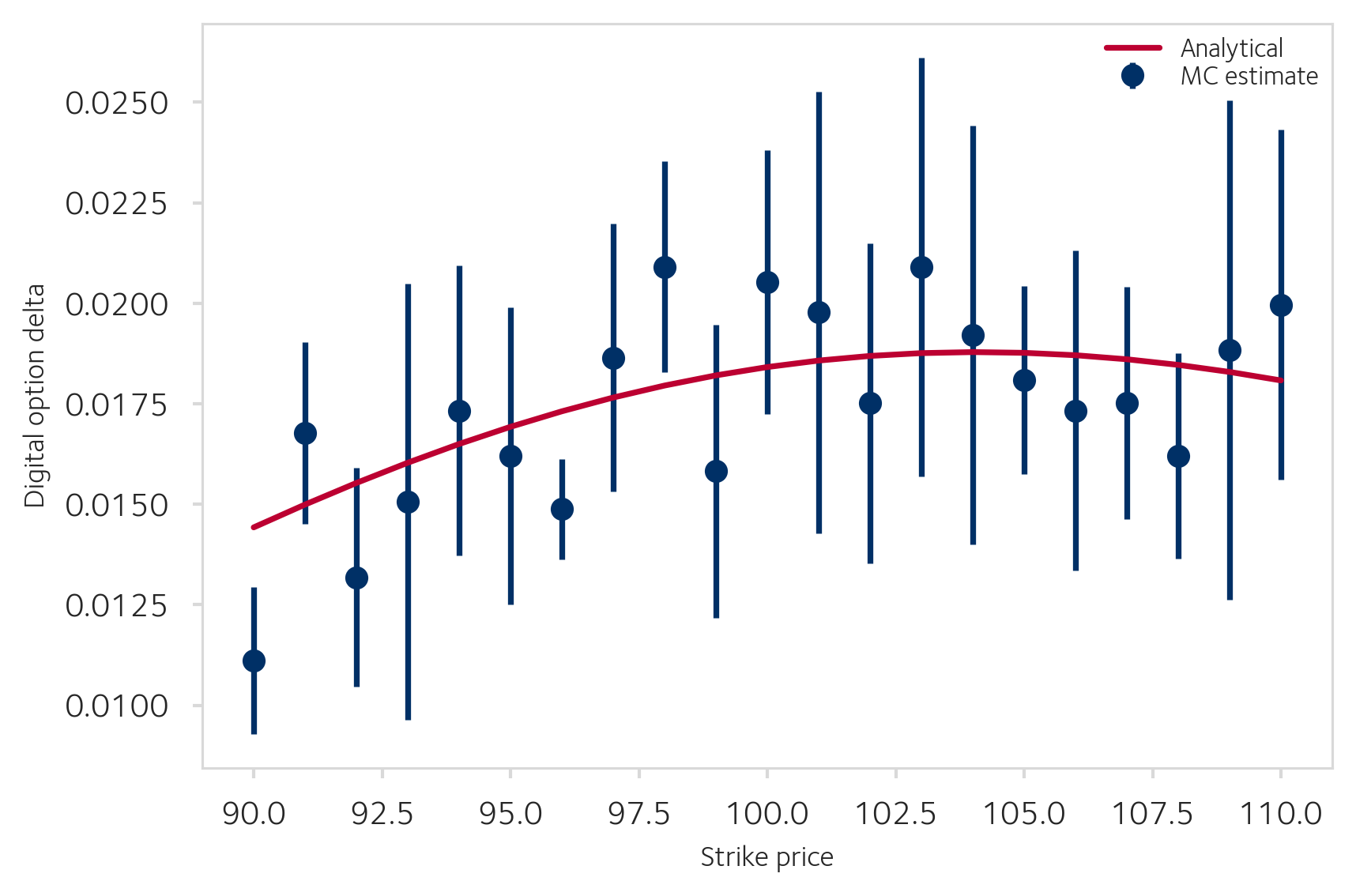
Digital Option Delta

A digital (binary) call pays 1 if $S_T > K$ and 0 otherwise. The analytical delta is

$$\Delta_{\mathrm{digital}} = \frac{e^{-rT}\,n(d_2)}{\sigma\,S\,\sqrt{T}},$$

where $n(\cdot)$ is the standard normal density. The discontinuous payoff function produces noisy delta estimates via bump-and-revalue.

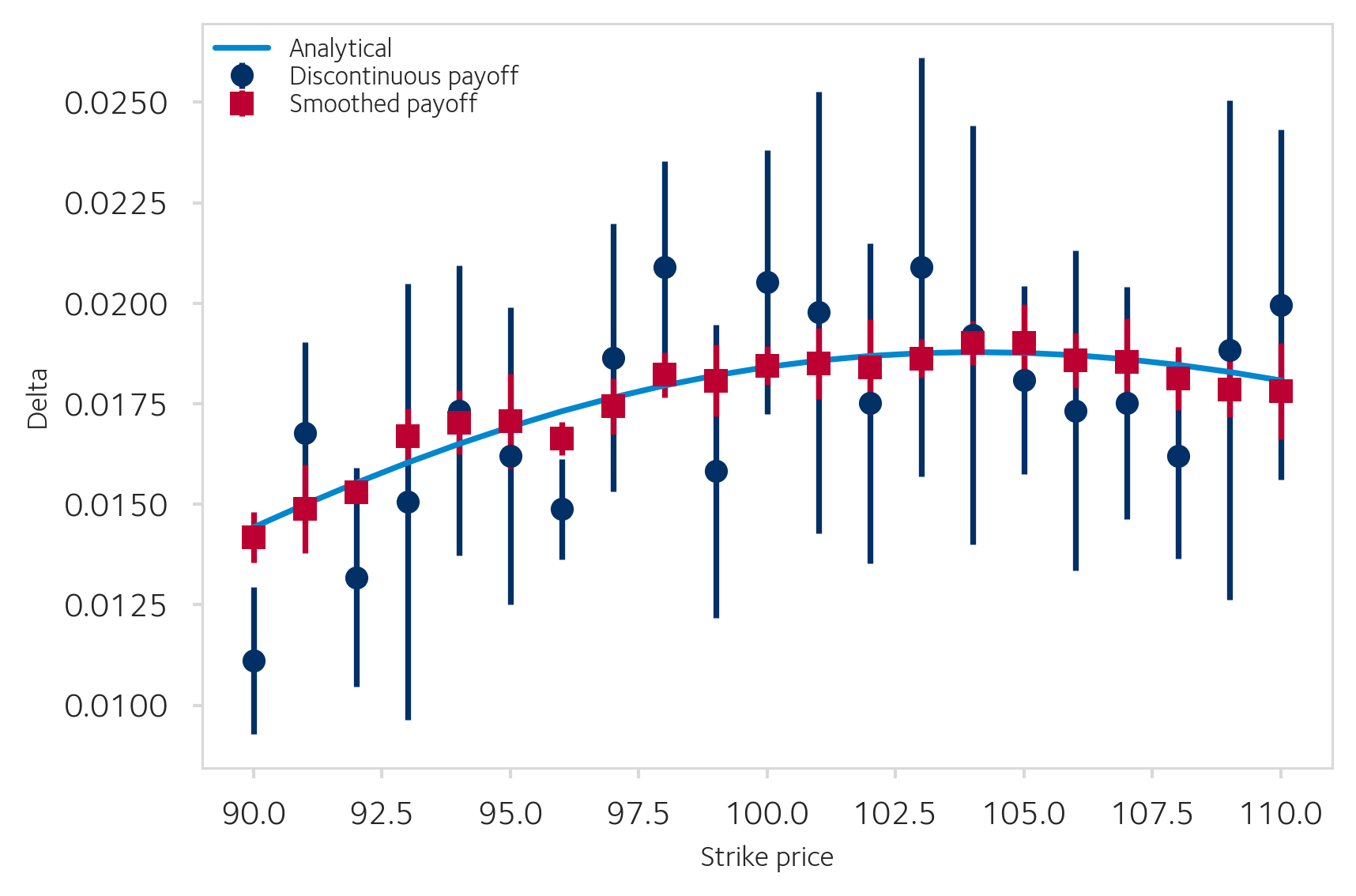
Smoothed Payoff

Replacing the discontinuous payoff with a logistic approximation $\frac{1}{1 + e^{-k(S_T - K)}}$ produces smoother delta estimates.

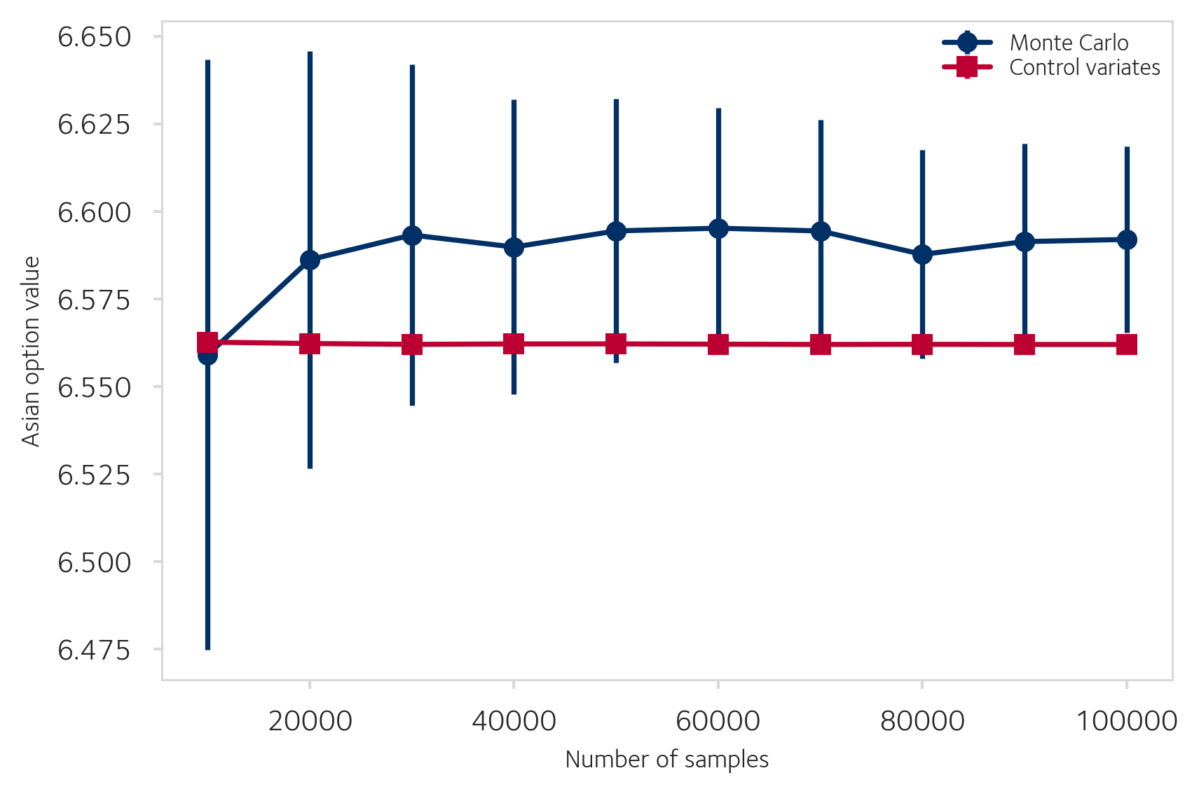
Variance Reduction for Asian Options

An Asian call option with arithmetic averaging has payoff $\max(\bar{A} - K, 0)$ where $\bar{A} = \frac{1}{N}\sum_{i=1}^{N} S_{t_i}$. No closed-form solution exists for the arithmetic average case.

Control Variates

The geometric-average Asian option $\tilde{A} = \left(\prod_{i=1}^{N} S_{t_i}\right)^{1/N}$ does admit an analytical price:

$$V_{\mathrm{geo}} = e^{-rT}\left[S_0\,e^{A + B^2/2}\,N(c + B) - K\,N(c)\right],$$

where $A = (r - \sigma^2/2)\,T/2$, $B = \sigma\sqrt{T}\sqrt{(2N+1)/(6(N+1))}$, and $c = (\ln(S_0/K) + A)/B$.

Using the geometric average payoff as a control variate with optimal $\beta$:

$$\hat{V}_{\mathrm{CV}} = \hat{V}_{\mathrm{arith}} - \beta\left(\hat{V}_{\mathrm{geo}} - V_{\mathrm{geo}}^{\mathrm{analytical}}\right).$$

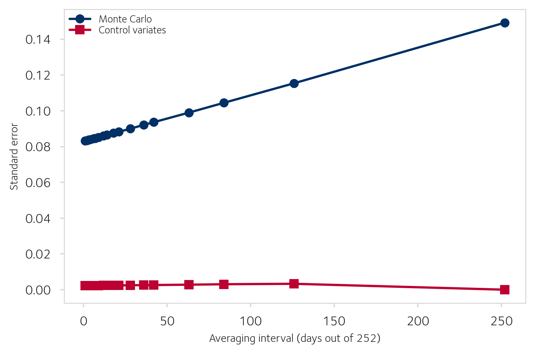
Asian Option: Standard Error Analysis