Building a Maximally Diversified Portfolio
Adapted from a chapter of my undergraduate dissertation, “Solving Financial Problems using Algorithmic Graph Theory” (2013).
The Problem
In the Capital Asset Pricing Model the risk of holding a portfolio splits into two kinds. Systematic risk is the risk shared by every stock in a market, sector, or whole financial system. Unsystematic (or idiosyncratic) risk is specific to one asset. Exposure to unsystematic risk can be reduced by diversifying, and a portfolio is more diversified when the stocks added to it are uncorrelated with the stocks already in it.
So the maximally diversified portfolio problem is: find a large set of stocks that are mutually uncorrelated.
A Correlation Graph
Take stocks and the matrix of pairwise correlations. Fix a maximum accepted correlation . Build a graph whose vertices are the stocks, joining two stocks with an edge whenever their correlation is at most , that is, whenever they are acceptably uncorrelated.
For the correlation itself we use the Pearson correlation of the two discrete-time price signals and over :
In this graph a valid portfolio is a set of stocks that are all pairwise uncorrelated, a set of vertices that are all mutually adjacent. That is a clique, and the largest such portfolio is a Maximum Clique.
The same problem has a mirror image. Build the complement graph instead, joining two stocks when they are too correlated (). Now a diversified portfolio is a set with no edges between any of its members, a Maximum Independent Set. The two formulations are complementary: a clique in one graph is an independent set in the other, and the complement is generated in time by inverting every entry of .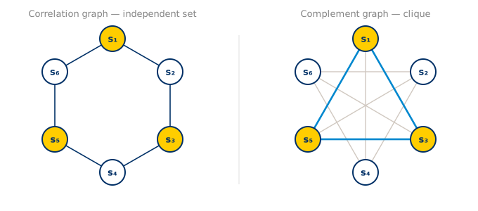
Complexity
Both Maximum Clique and Maximum Independent Set are NP-hard optimisation problems. A graph can have up to maximal cliques, so any method that enumerates them all is exponential in the worst case.
Exact: Bron-Kerbosch
The Bron-Kerbosch algorithm enumerates every maximal clique. It carries three sets: , the clique built so far; , the candidates that extend it; and , vertices already processed.
function BronKerbosch(R, P, X):
    if P = ∅ and X = ∅:
        emit(R)                       # R is a maximal clique
    else:
        for each v in P:
            BronKerbosch(R ∪ {v},
                         P ∩ neighbours(v),
                         X ∩ neighbours(v))
            P ← P − {v}
            X ← X ∪ {v}
The initial call is BronKerbosch(∅, V, ∅). A clique is recorded when there are no candidates left and no already-processed vertices that could extend it. At each step a vertex is added to , the candidate set is narrowed to so that everything stays mutually connected, and afterwards moves from into . The algorithm enumerates all cliques in time linear in their number, and since that number is exponential it runs in .
Approximate: Halldórsson-Boppana
For thousands of stocks, exhaustive enumeration is hopeless, so we also implement the Halldórsson-Boppana approximation, which approximates the Maximum Independent Set (and by complement the Maximum Clique) within a factor of . It is built from two routines. Ramsey recursively splits the graph at a vertex into its neighbours and non-neighbours, returning a clique and an independent set:
function Ramsey(G):
    if G = ∅:
        return (∅, ∅)
    choose some v in V
    (C1, I1) ← Ramsey(Neighbours(v))
    (C2, I2) ← Ramsey(NonNeighbours(v))
    return ( largest(C1 ∪ {v}, C2),
             largest(I1, I2 ∪ {v}) )
CliqueRemoval repeatedly strips a clique returned by Ramsey and keeps the best independent set found across the rounds:
function CliqueRemoval(G):
    i ← 1
    (C_i, I_i) ← Ramsey(G)
    while G ≠ ∅:
        G ← G − C_i
        i ← i + 1
        (C_i, I_i) ← Ramsey(G)
    return ( max over j of I_j, {C_1, C_2, … C_i} )
Dataset and Results
The correlations were computed over 475 of the 500 stocks in the S&P 500, from 2013-01-01 to 2013-07-01, using the Pearson function above. The correlation matrix had mean and standard deviation . From it we generated three graphs, at correlation thresholds , , and , with the density of a graph defined as
Because the mean correlation is , a low threshold admits very few pairs (the graph is sparse), while a threshold near the mean admits roughly half of all pairs. At the graph has edges on vertices, a density of about . For each graph we ran Bron-Kerbosch (recording the largest clique and the time) and the Halldórsson-Boppana approximation (best clique over 10 runs, averaged time).
| Threshold | Density | Bron-Kerbosch size | BK time | Halldórsson-Boppana size | H&B time |
|---|---|---|---|---|---|
| 0.1 | 0.08 | 15 | 5.4 s | 2 | 6.6 s |
| 0.2 | 0.26 | 49 | 27 min | 4 | 5.8 s |
| 0.3 | 0.46 | 62 | 2 h | 5 | 8.2 s |
There is no single best method. Bron-Kerbosch finds large cliques quickly on sparse graphs but becomes infeasible as density grows, taking two hours at . The approximation is fast and its runtime barely moves with density, but it returns cliques of size 2 to 5, which is useless here: the literature suggests around 30 stocks are needed to diversify away most idiosyncratic risk. If an investor is restricted to the S&P 500, the only way to obtain a portfolio of usable size is exhaustive enumeration, paid for in computation time.
How Much of This Is Noise?
There is a bridge between this combinatorial picture and the spectral one. Suppose the correlation matrix were pure noise, with its eigenvalues filling the Marchenko-Pastur sea. Thresholding it at would then, to first order, produce an Erdős-Rényi graph with edge probability under the null. Erdős-Rényi graphs have a sharply concentrated clique number of about , only logarithmic in . That gives a free null model for the table above. At and , so , noise alone would yield cliques of about 16, where we found 62. A clique that large cannot be explained by noise, so it is reporting genuine correlation structure.
What lifts the real cliques above that noise floor is the handful of eigenvalues that stand outside the Marchenko-Pastur sea: the market mode, in which everything co-moves, and the sector modes. Random matrix theory is the spectral view of the same block structure that Bron-Kerbosch hunts for combinatorially. The connection runs deeper than an analogy. A correlated sector is a planted dense subgraph, and the planted-clique problem says such a block is detectable cheaply from the leading eigenvector once it is larger than about , but is conjectured to be combinatorially hard below that size. Cleaning the matrix with random matrix theory first is therefore not just hygiene. It is the cheap spectral relaxation of the same NP-hard clique problem we then solve by brute force, and the gap between and is this post’s exact-versus-approximate tension seen from the spectral side.
Takeaways
- Diversification has a clean combinatorial core: a maximally diversified portfolio is a Maximum Clique in a correlation-threshold graph (equivalently a Maximum Independent Set in its complement).
- That core is NP-hard, and the practical tension is the usual one. Exact enumeration gives portfolios large enough to matter but does not scale; the polynomial approximation scales but returns sets too small to diversify.
- On a universe the size of the S&P 500, exhaustive Bron-Kerbosch is still the only thing that produces a portfolio worth holding.
This is the second of three problems from the dissertation. The others recast debt resolution and currency arbitrage as graph problems in the same way.
References
- C. Bron and J. Kerbosch (1973). Algorithm 457: Finding All Cliques of an Undirected Graph. Communications of the ACM 16(9).
- J. W. Moon and L. Moser (1965). On Cliques in Graphs. Israel Journal of Mathematics 3. Establishes the bound on maximal cliques.
- R. Boppana and M. M. Halldórsson (1992). Approximating Maximum Independent Sets by Excluding Subgraphs. BIT 32(2).
- M. Statman (1987). How Many Stocks Make a Diversified Portfolio? Journal of Financial and Quantitative Analysis 22(3).
- L. Laloux, P. Cizeau, J.-P. Bouchaud, and M. Potters (1999). Noise Dressing of Financial Correlation Matrices. Physical Review Letters 83(7). Random matrix theory applied to the correlation matrix.
- N. Alon, M. Krivelevich, and B. Sudakov (1998). Finding a Large Hidden Clique in a Random Graph. The spectral threshold for the planted-clique problem.