Mandelbrot Set: Shallow-Regime Sampling Optimizations
The Escape-Time Algorithm and Its Bottleneck
The standard escape-time algorithm iterates starting from . If for some , the orbit escapes and is colored by the escape iteration count. If the orbit survives to a cap , the pixel is colored black — the point is treated as interior.
Interior points are the expensive case: every one runs to the cap. In a shallow-regime render (full-set views, zoom depths where double precision holds) the typical iteration cap is a few hundred to a few thousand. If a large fraction of pixels land inside the set, those pixels dominate the total work budget.
The leverage is a conservative interior predicate — a cheap test that proves a point is inside:
The predicate is allowed to miss interior points (false negatives fall through to escape-time at no extra cost), but must never claim an exterior point is interior (a false positive would mis-color a pixel). This asymmetry is the whole design.
We build three layers, ordered by cost and coverage.
Layer 1: Main Cardioid (Exact)
The main cardioid is the set of for which has an attracting fixed point. A fixed point satisfies with multiplier ; attracting means . Parametrizing by the multiplier:
To test membership we invert: the fixed point is and the interior condition is . The complex square root can be eliminated. With
the cardioid interior is exactly the set where
This is not an approximation — it is the exact interior. It costs four multiplications and two additions per point.
Layer 2: Period-2 Disk (Exact)
The genuine period-2 points satisfy . The degree-4 polynomial factors as , where the first factor gives the 2-cycle after dividing out fixed points. By Vieta’s formulas the product of the two 2-cycle elements is , and the 2-cycle multiplier is
Since is linear in , the interior maps to an exact disk:
Period 2 is the only nontrivial hyperbolic component whose multiplier is linear in . Every higher-period component has a nonlinear multiplier-to-parameter map, so none of them is an exact disk in the -plane.
Layer 3: Period-3 Bulbs (Inscribed Disks, MC-Calibrated)
The period-3 superattracting parameters — where lies on the 3-cycle, — are roots of
One root is real (, on the antenna); the conjugate pair () sits on the two round bulbs attached to the main cardioid. The boundaries of these bulbs are not circles — their exact boundary is determined by a degree-9 resultant in — so we inscribe a disk at each center instead.
The inscribed radius must be backed off below the geometric inscribed radius, or the test stops being conservative near the curved boundary. Rather than deriving the exact inscribed radius analytically, we measure a safe lower bound by Monte Carlo:
- Draw 1.5 million random samples from the bounding box .
- Run escape-time with to classify each sample as interior or escaping.
- For each period-3 center, record the minimum distance to any escaping sample. This is a stochastic lower bound on the true inscribed radius.
- Apply a safety shrink factor to that lower bound.
The antenna center admits only a tiny disk (the filament region is spiky, so escaping points are nearby). The two cardioid-attached bulbs give usable disks:
| Center | MC lower bound | Used radius () |
|---|---|---|
The antenna center yields , below the 0.02 threshold used to filter out negligible disks.
Visual Confirmation
The figure below renders the set with log-scaled escape-time coloring and overlays the three analytic regions. The period-3 inscribed disks sit visibly inside their bulbs with margin to spare.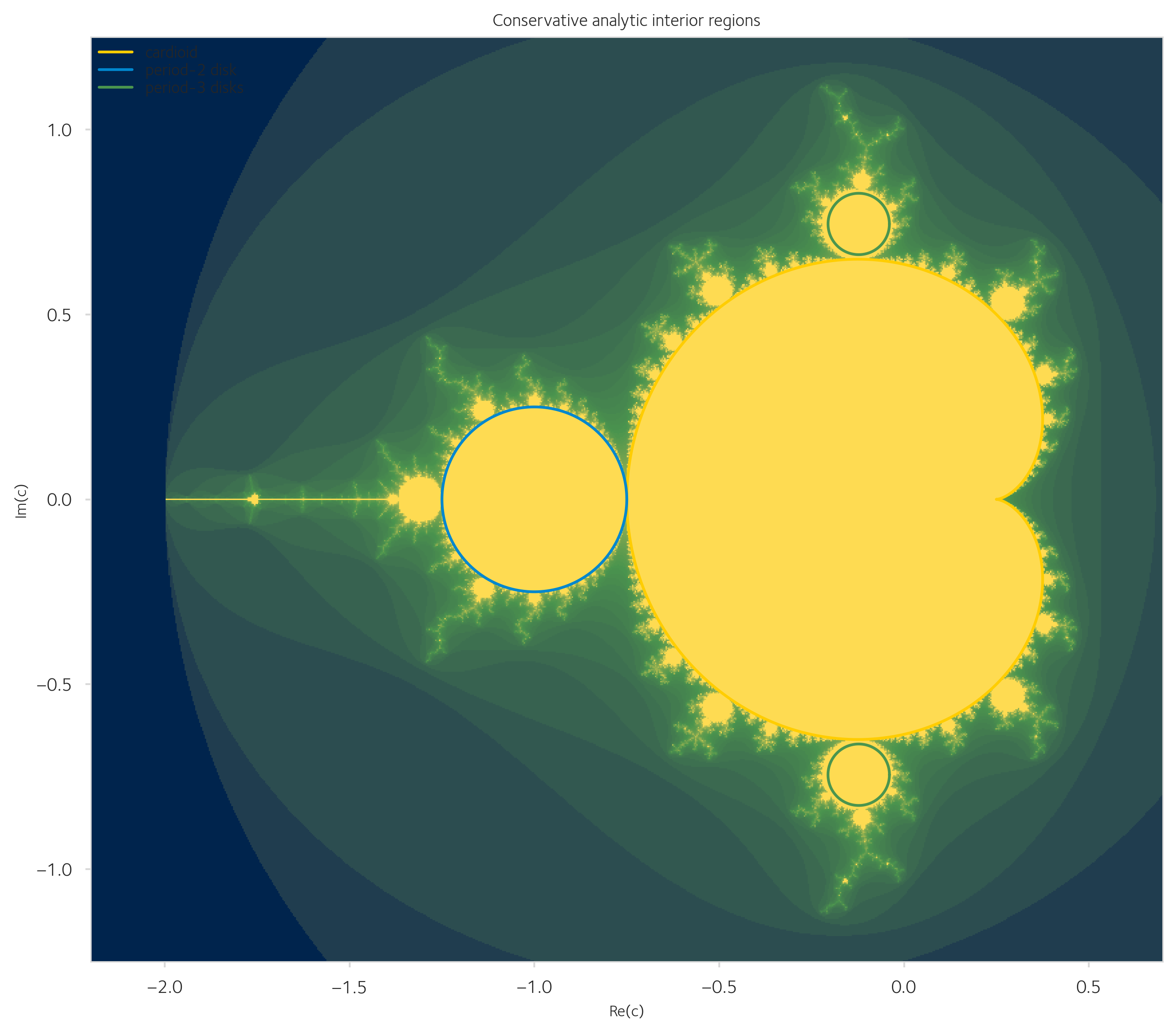
Conservativeness and Coverage
We verify on a fresh 3-million-point random sample (bounding box , ) that no layer produces false positives, then measure interior coverage:
| Predicate | Interior caught | False positives |
|---|---|---|
| cardioid | ~78% | 0 |
| cardioid + period-2 | ~91% | 0 |
| cardioid + period-2 + period-3 | ~94% | 0 |
The cardioid alone captures roughly three-quarters of all interior mass. Adding the period-2 disk crosses 90%. The period-3 disks add a few more percentage points. The long tail of smaller bulbs is deliberately left to escape-time.
If period-3 shows false positives, the shrink factor is too loose — reduce SHRINK until the count reaches zero.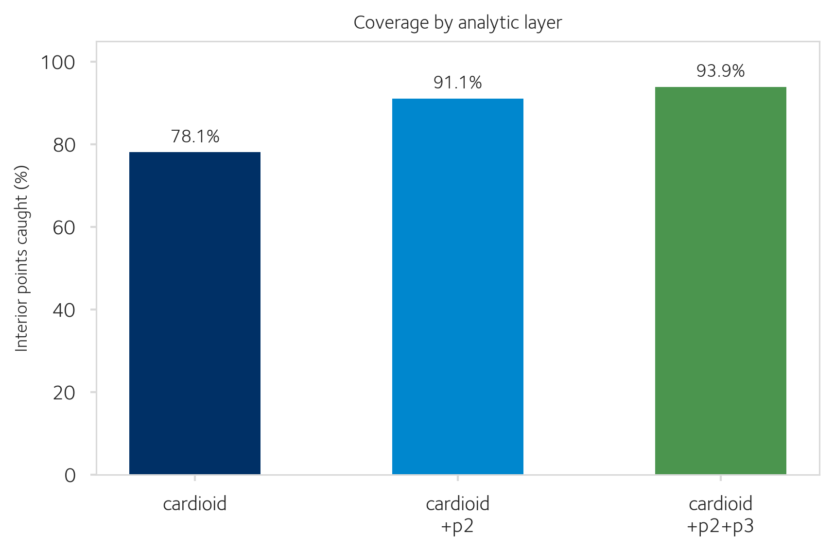
Iteration-Work Savings
Coverage of interior mass understates the true benefit: interior points are exactly the expensive ones, each costing iterations. We model work explicitly:
- Baseline: every point costs its escape-time iteration count; interior points cost .
- With tests: points caught by the predicate cost a small constant (about 4 comparison operations); everyone else is unchanged.
On the 3-million-point sample with :
The exact figure depends on what fraction of the bounding box is interior, which varies with the view. Full-set views have higher interior fraction and therefore larger savings; deep zooms into exterior spirals have near-zero interior fraction and therefore near-zero benefit from these tests.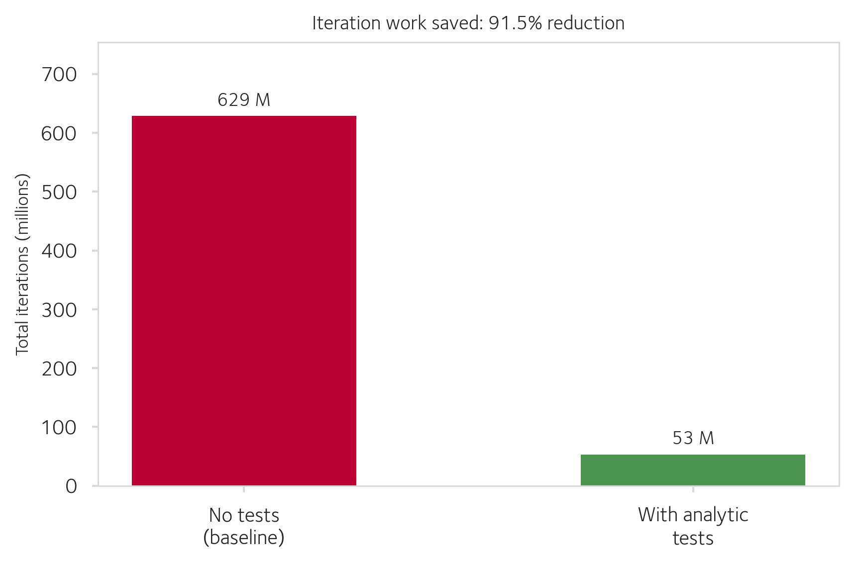
Design Notes
Why not use larger disks? The period-3 boundary is curved and the inscribed disk underestimates the component. The shrink factor is the margin of safety. A tighter MC sample (more points, higher ) converges the lower bound upward, allowing a slightly larger disk, but the gain diminishes quickly.
Why stop at period 3? The inscribable disk radius shrinks roughly as along the Mandelbrot boundary for period- components, and filament-region components admit almost no inscribed disk at all (the antenna period-3 center above). Past period 3 the per-branch overhead exceeds the iteration savings.
Clean handoff. These tests handle the large round interior components. Everything else — fine filament structures, higher-period bulbs, deep zooms — is handled by escape-time plus periodicity detection (Brent’s cycle detection, or atom-domain tests). The two methods are complementary and compose without interaction.
Deep-zoom regime. In the deep-zoom regime the interior-skipping question becomes secondary to a different bottleneck: double precision no longer resolves the structure, and per-pixel extended-precision arithmetic dominates the budget. The analytic tests remain valid (the cardioid and period-2 disk are exact in exact arithmetic) but the savings they provide are negligible relative to the precision cost.