Adapted from a 2015 computational finance assignment. It prices the same European call as the Monte Carlo and COS-method posts.

The Equation on a Grid

The value $V(S,t)$ of a European option under Black-Scholes obeys

$$\frac{\partial V}{\partial t} + rS\frac{\partial V}{\partial S} + \tfrac{1}{2}\sigma^2 S^2\frac{\partial^2 V}{\partial S^2} = rV.$$

Monte Carlo integrates the terminal payoff over simulated paths; the COS method integrates it against the characteristic function. The finite-difference method discretises the equation itself onto a grid in price and time and marches the payoff at expiry backwards to today. The payoff is the terminal condition, so time runs in reverse. Write

$$\tau = T - t,$$

so the payoff sits at $\tau = 0$ and the solution advances in $\tau$. With $\Theta = \partial V/\partial t$, $\Delta = \partial V/\partial S$, $\Gamma = \partial^2 V/\partial S^2$, the equation is $\Theta + rS\Delta + \tfrac12\sigma^2 S^2\Gamma = rV$. Throughout, the option is a European call with $K = 110$, $T = 1$, $\sigma = 0.30$, $r = 0.04$; its analytical value at $S_0 = 100$ is $9.6254$.

Two Grids

There are two standard choices of spatial grid.

The untransformed grid places nodes at $S_i = i\,\delta S$, evenly spaced in price. The PDE keeps its $S$-dependent coefficients $rS$ and $\tfrac12\sigma^2 S^2$.

The log grid changes variables to $x = \ln S$. Substituting $x = \ln S$ and $\tau = T-t$ and writing $U(x,\tau) = V(S,t)$ gives

$$\frac{\partial U}{\partial \tau} = \tfrac{1}{2}\sigma^2\frac{\partial^2 U}{\partial x^2} + \left(r - \tfrac{1}{2}\sigma^2\right)\frac{\partial U}{\partial x} - rU.$$

The diffusion and drift coefficients are now constant in $x$. Equal steps in $x$ are geometric steps in $S$: the grid is fine at small $S$, and a distant upper boundary costs few extra nodes.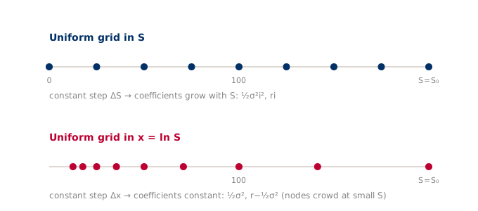

Each grid has its own coefficients: $rS$ and $\tfrac12\sigma^2 S^2$ on the $S$ grid, the constants $(r - \tfrac12\sigma^2)$ and $\tfrac12\sigma^2$ on the log grid. The scheme below uses the $S$ grid.

The Stencils

The three derivatives are replaced by difference quotients from Taylor expansions. These are the same on either grid. For $\Theta$, a forward Euler step in time. Expanding $V(S, t - \delta t)$ about $(S,t)$,

$$\frac{\partial V}{\partial t}(S,t) = \frac{V(S,t) - V(S, t-\delta t)}{\delta t} + \mathcal{O}(\delta t).$$

On the grid, with time indexed by $\tau$ so that a higher index is an earlier calendar time, and $V^n_i$ the value at node $i$ and step $n$, this is $(V^n_i - V^{n+1}_i)/\delta t$.

For $\Delta$, a centred difference. The two expansions

$$V(S \pm \delta S, t) = V(S,t) \pm \delta S\, \frac{\partial V}{\partial S} + \tfrac12\delta S^2\frac{\partial^2 V}{\partial S^2} + \mathcal{O}(\delta S^3)$$

subtract to cancel the even terms:

$$\frac{\partial V}{\partial S}(S,t) = \frac{V^n_{i+1} - V^n_{i-1}}{2\,\delta S} + \mathcal{O}(\delta S^2).$$

Adding the same two expansions cancels the odd terms and gives $\Gamma$:

$$\frac{\partial^2 V}{\partial S^2}(S,t) = \frac{V^n_{i+1} - 2V^n_i + V^n_{i-1}}{\delta S^2} + \mathcal{O}(\delta S^2).$$

FTCS: the Explicit Scheme

Forward-Time Centred-Space substitutes the three stencils into the PDE and solves for the single unknown $V^{n+1}_i$ from three known values at the previous step. On the $S$ grid, because $S_i = i\,\delta S$ the factor $\delta S$ cancels against the $S$ and $S^2$ in the coefficients, and the update reduces to functions of the index $i$:

$$V^{n+1}_i = a_i V^n_{i-1} + b_i V^n_i + c_i V^n_{i+1},$$

$$a_i = \tfrac12(\sigma^2 i^2 - r i)\,\delta t,\quad b_i = 1 - (\sigma^2 i^2 + r)\,\delta t,\quad c_i = \tfrac12(\sigma^2 i^2 + r i)\,\delta t.$$

Each new value is computed directly, with no system to solve.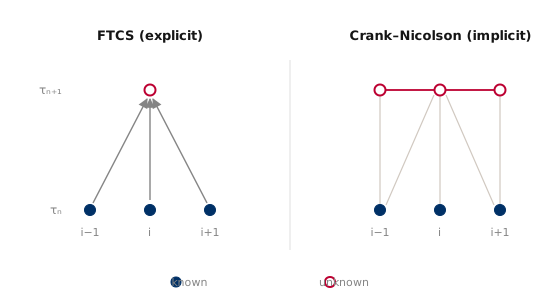

An easy thing to get wrong. The coefficients $a_i, b_i, c_i$ carry the factors $\sigma^2 i^2$ and $r i$, which are the $S$-grid coefficients $\tfrac12\sigma^2 S_i^2$ and $rS_i$ with the $\delta S$ divided out. It is tempting to use the log-grid constants $(r - \tfrac12\sigma^2)$ and $\tfrac12\sigma^2$ here instead. This is what I did on my first attempt, in the computational finance course where I met these methods. Consider the diffusion term at $S = 100$: on the $S$ grid it is $\tfrac12\sigma^2 S^2 = 0.045 \times 10^4 = 450$, while the log-grid constant $\tfrac12\sigma^2 = 0.045$ is smaller by a factor of $10^4$. With the constant on the $S$ grid the diffusion is far too small, value does not spread inward from the in-the-money region, and the out-of-the-money call is priced at essentially zero: the scheme returns $0.0001$ for the $9.6254$ call. The constants are correct on the log grid, where the payoff is $\max(e^{x_i} - K, 0)$ and the step is $\delta x$. On the $S$ grid the coefficients depend on $S$.

Stability

The explicit scheme is only conditionally stable. The binding requirement is $b_i \ge 0$, worst at the top of the grid where $i$ is largest:

$$\delta t \le \frac{1}{\sigma^2 i_{\max}^2 + r} \approx \frac{1}{\sigma^2 N^2}.$$

The timestep must shrink like $1/N^2$. Doubling the asset resolution quadruples the number of timesteps: $N = 20$ needs $40$ steps, $N = 100$ needs $1000$, $N = 200$ needs $4000$. The work grows like $N^3$. This is the main drawback of the explicit scheme, and the reason for the implicit scheme below.

Crank-Nicolson: the Implicit Scheme

Crank-Nicolson averages the spatial operator over the old and new time levels. Writing the discretised right-hand side of the PDE as a tridiagonal operator $\mathcal{L}$ acting on the value vector, the update is

$$\left(I - \tfrac12\delta t\,\mathcal{L}\right)V^{n+1} = \left(I + \tfrac12\delta t\,\mathcal{L}\right)V^n.$$

Now $V^{n+1}$ appears on both sides. The three unknowns at each step are coupled, and each step solves a tridiagonal system by one LU (or Thomas) sweep in $\mathcal{O}(N)$. Crank-Nicolson is unconditionally stable, so the timestep is set by accuracy rather than stability, and its error is $\mathcal{O}(\delta t^2 + \delta S^2)$ against the explicit scheme’s $\mathcal{O}(\delta t + \delta S^2)$. The matrix should be factored once and the factorisation reused each step; re-inverting it every timestep costs $\mathcal{O}(N^3)$ per step.

Boundary Conditions

The grid is finite, so the scheme needs values at the edges. For a call:

• At $S = 0$ the option is worthless: $V(0, \tau) = 0$.
• As $S \to \infty$ the call approaches the forward: $V(S_{\max}, \tau) = S_{\max} - K e^{-r\tau}$, the stock minus the discounted strike. An alternative is the linearity condition $\Gamma = 0$, imposed as $V_N = 2V_{N-1} - V_{N-2}$.

The upper condition is only asymptotic, and imposing it at a finite $S_{\max}$ introduces an error. At a modest boundary the true value still sits below $S_{\max} - K e^{-r\tau}$, since the option retains some time value and its delta is below one. Pinning the boundary above the true value biases the solution upward, and refining the grid does not remove the error. Placing the boundary at several times the strike keeps it negligible.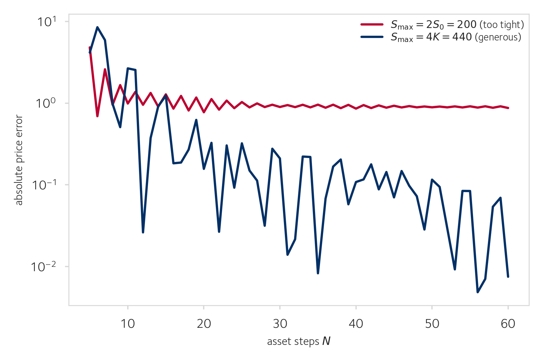

Results

With a generous domain, both schemes converge to the analytical value as the grid is refined. Convergence is oscillatory: the node nearest the spot straddles it alternately from above and below as $N$ change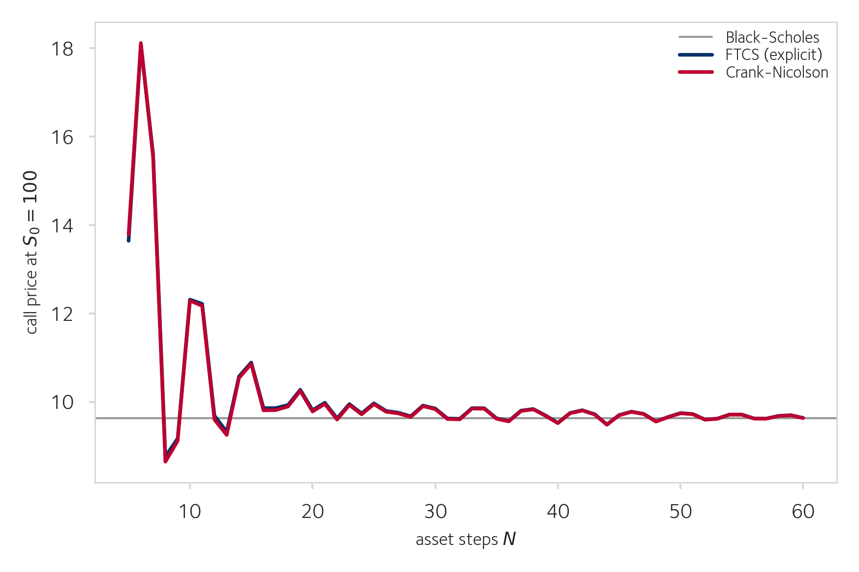s.

The overlap is expected, not a shortcoming of Crank-Nicolson. At a fixed asset grid both schemes carry the same $\mathcal{O}(\delta S^2)$ spatial error, and the plot runs each with enough timesteps that the time error is negligible, so they reach the same value. The schemes differ in the cost of getting there. FTCS is stable only for $\delta t \lesssim 1/(\sigma^2 N^2)$, so its number of timesteps must grow like $N^2$; Crank-Nicolson is unconditionally stable and needs only $M \sim N$ steps for comparable time accuracy. At $N = 100$ that is about $1000$ steps against $100$, and the gap widens with resolution.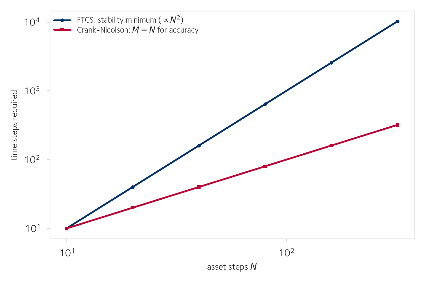

At $N = 100$ both schemes agree with Black-Scholes across moneyness:

The grid also gives the Greeks, as differences of the value surface it already holds. A centred difference of the solution gives the delta across the range of $S$ without further solving.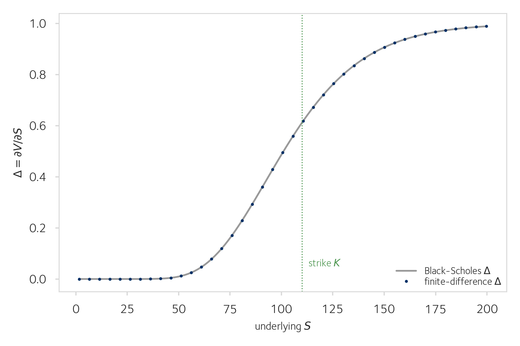

Summary

The finite-difference method prices the option by discretising the Black-Scholes PDE and marching the payoff backwards, producing the value surface and the Greeks from one solve. At a given asset grid the explicit and implicit schemes return the same price, set by the shared spatial error; they differ in cost. FTCS is conditionally stable, so its number of timesteps grows like $N^2$. Crank-Nicolson is unconditionally stable and second order in time, needing only $M \sim N$ steps, at the cost of a tridiagonal solve per step. Two choices matter as much as the scheme: the grid, whose coefficients must match the transform, and the placement of the far boundary.