Characteristic Function Approach

Under geometric Brownian motion, the log-price increment $\ln(S_T/K)$ has a known characteristic function. Rather than working with the probability density directly, we exploit the fact that any density $f(x)$ on a finite interval $[a, b]$ admits a Fourier cosine expansion

$$f(x) = \frac{2}{b - a} \sum_{k=0}^{\infty}{}' A_k \cos\!\left(\frac{k\pi(x - a)}{b - a}\right),$$

where the prime denotes that the first term is halved, and

$$A_k = \int_a^b f(x) \cos\!\left(\frac{k\pi(x - a)}{b - a}\right) dx.$$

The key insight is that $A_k$ can be recovered from the characteristic function $\phi(u) = \mathbb{E}[e^{iux}]$ without knowing $f$ explicitly:

$$A_k \approx \operatorname{Re}\!\left[\phi\!\left(\frac{k\pi}{b - a}\right) e^{-i\frac{k\pi a}{b - a}}\right].$$

For the GBM model, the characteristic function of $x = \ln(S_T/K)$ is

$$\phi(u) = \exp\!\left[iu\!\left(r - \tfrac{1}{2}\sigma^2\right)\!\tau - \tfrac{1}{2}\sigma^2\tau\, u^2\right].$$

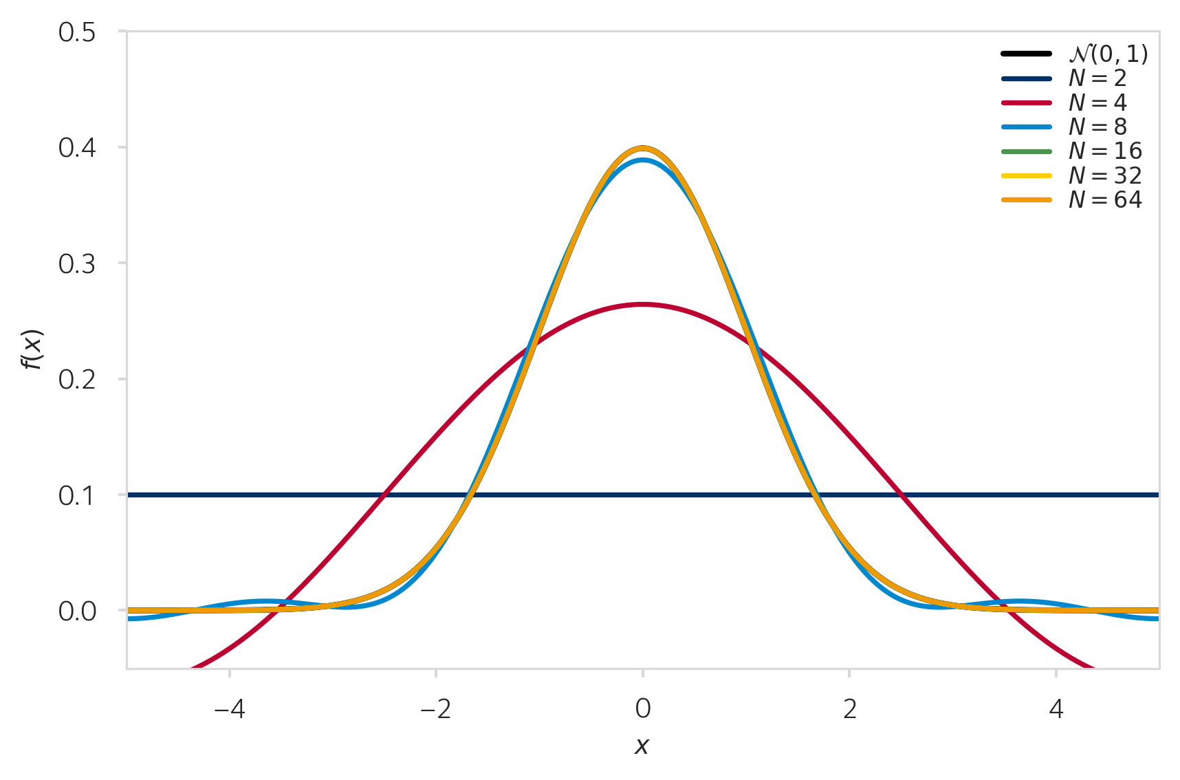
The cosine expansion converges rapidly for smooth densities. With only a handful of terms, the standard normal density is already well approximated.

Chi and Psi Coefficients

The option price requires computing the inner product of the density coefficients $F_k$ with the payoff coefficients $V_k$. The payoff coefficients decompose into two integrals, $\chi_k$ and $\psi_k$, that can be evaluated in closed form.

The $\chi_k$ coefficient captures the exponential part of the payoff:

$$\chi_k(c, d) = \int_c^d e^x \cos\!\left(\frac{k\pi(x - a)}{b - a}\right) dx = \frac{1}{1 + u_k^2}\left[\cos(u_k(d - a))\,e^d - \cos(u_k(c - a))\,e^c + u_k\sin(u_k(d - a))\,e^d - u_k\sin(u_k(c - a))\,e^c\right],$$

where $u_k = \frac{k\pi}{b - a}$.

The $\psi_k$ coefficient captures the constant part:

$$\psi_k(c, d) = \int_c^d \cos\!\left(\frac{k\pi(x - a)}{b - a}\right) dx = \begin{cases} d - c & k = 0 \\ \frac{\sin(u_k(d - a)) - \sin(u_k(c - a))}{u_k} & k > 0. \end{cases}$$

The integration limits $(c, d)$ depend on the option type: $(0, b)$ for calls and $(a, 0)$ for puts.

Truncation Range

The cosine expansion requires a finite domain $[a, b]$. This range must be wide enough to capture the mass of the density, but not so wide that the cosine basis functions oscillate excessively relative to the number of terms $N$.

Two formulations appear in the literature. The first centres the range on the forward:

$$a, b = \ln(S_0/K) + r\tau \mp L\sqrt{\sigma^2 \tau},$$

and the second uses the first cumulant (the mean of the log-price increment):

$$a, b = \ln(S_0/K) + \left(r - \tfrac{1}{2}\sigma^2\right)\tau \mp L\sqrt{\sigma^2 \tau},$$

where $L$ controls the number of standard deviations included. Both formulations converge, but the cumulant-based formula places the interval symmetrically around the true mean of the distribution, which leads to faster convergence at moderate $N$.

The COS Pricing Formula

Combining the density and payoff coefficients, the discounted option price is

$$V = e^{-r\tau} \sum_{k=0}^{N-1}{}' F_k \cdot V_k,$$

where

$$F_k = \operatorname{Re}\!\left[\phi\!\left(\frac{k\pi}{b - a}\right) e^{i\frac{k\pi}{b - a}(\ln(S_0/K) - a)}\right]$$

and

$$V_k = \frac{2}{b - a}\, K\, (\chi_k - \psi_k) \quad \text{(call)}, \qquad V_k = \frac{2}{b - a}\, K\, (\psi_k - \chi_k) \quad \text{(put)}.$$

The computational cost is $\mathcal{O}(N)$ per option price: all $N$ terms involve elementary trigonometric and exponential evaluations with no matrix inversions or root-finding. This makes the COS method substantially faster than PDE or Monte Carlo methods for European-style contracts.

Results

Price vs Spot

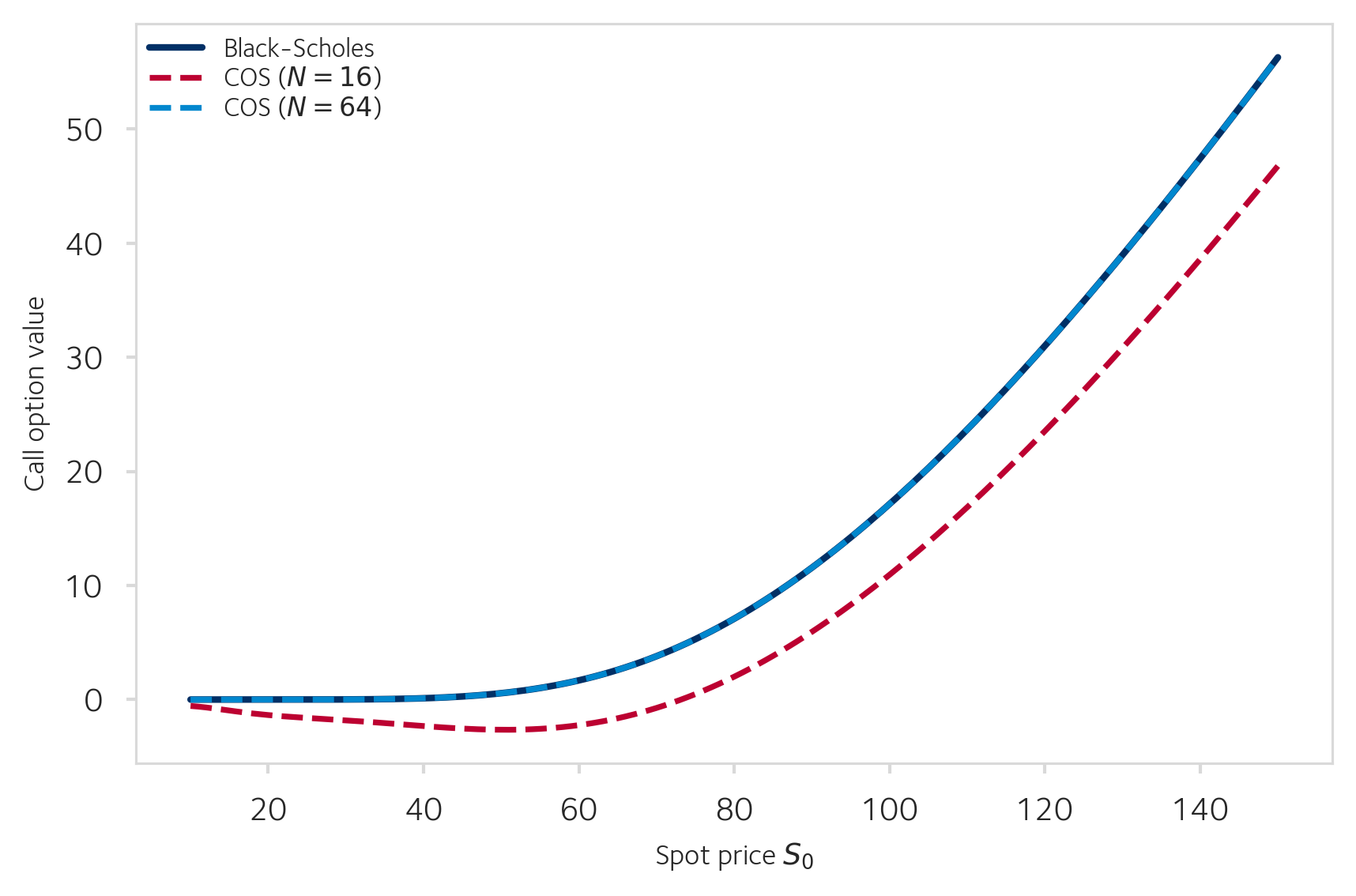
With $K = 100$, $r = 0.03$, $T = 1$, $\sigma = 0.40$, the COS price is compared against the analytical Black-Scholes price across a range of spot values. At $N = 16$ terms, the approximation deviates noticeably for deep out-of-the-money options where the truncation range $[a,b]$ (width $2L\sigma\sqrt{T} \approx 9.6$ with $L = 12$) demands more basis functions to resolve. At $N = 64$, the COS price is indistinguishable from the analytical result.

Convergence of the Relative Error

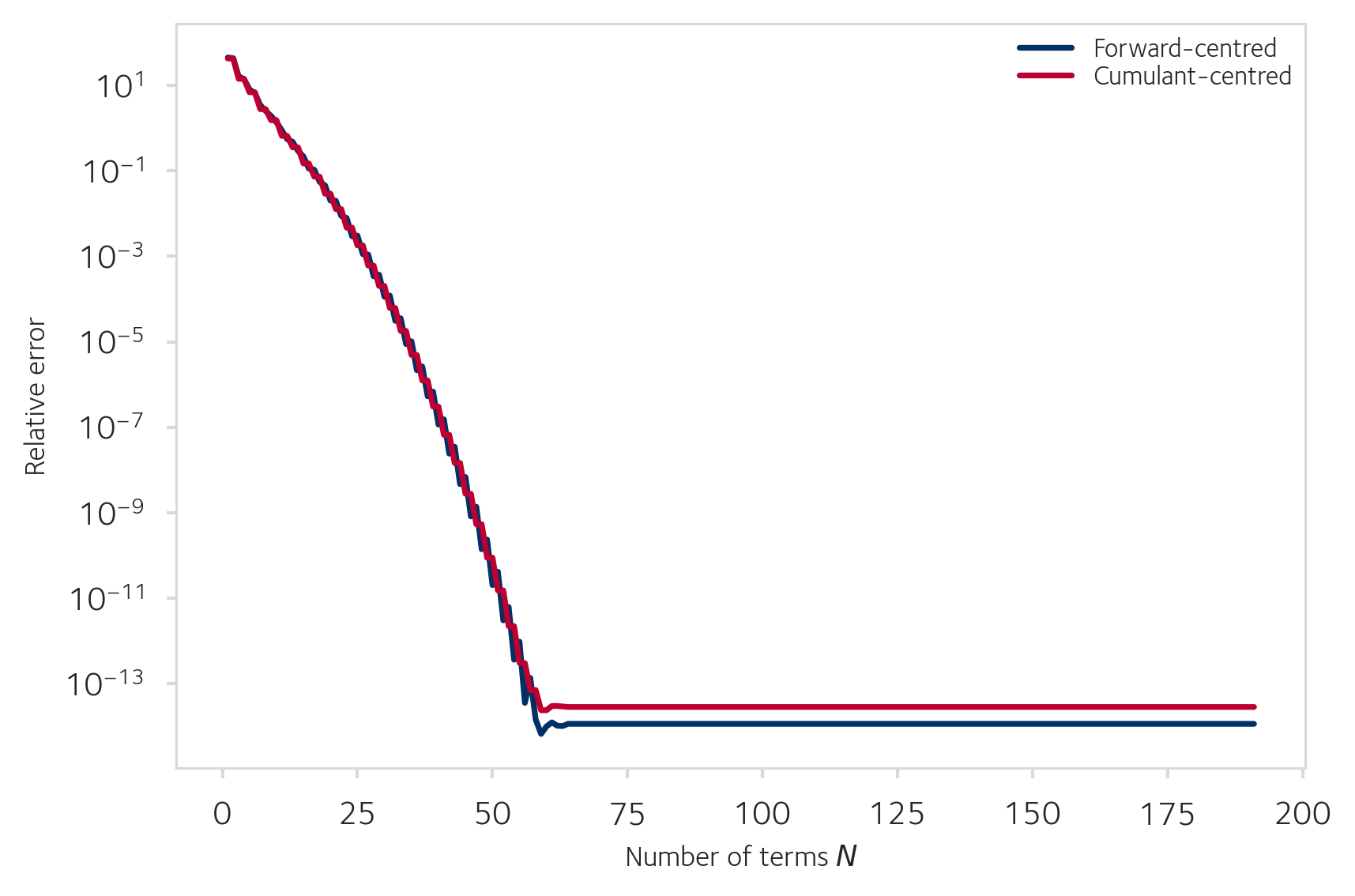
The relative error $|V_{\mathrm{COS}} - V_{\mathrm{BS}}| / V_{\mathrm{BS}}$ decreases exponentially as the number of terms $N$ grows, reaching machine precision around $N = 65$ for a standard GBM parameterisation ($S_0 = 100$, $K = 110$, $r = 0.04$, $T = 1$, $\sigma = 0.30$).

With $L = 12$, both truncation formulas converge at nearly the same rate. The difference between their centres ($0.5\sigma^2\tau$) is small relative to the total range width ($2L\sigma\sqrt{\tau}$), so the effect of mis-centring is negligible. With a smaller $L$, the cumulant-based formula would show a more pronounced advantage.

Value Convergence

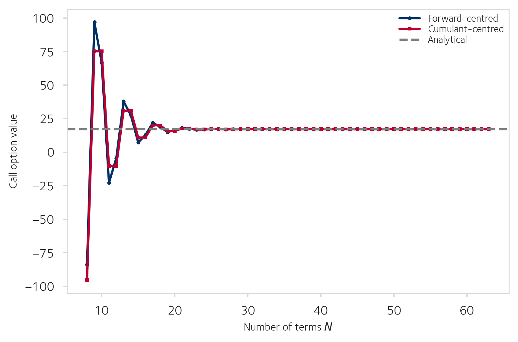
The raw option value oscillates at small $N$ but stabilises rapidly. For the at-the-money case ($S_0 = K = 100$, $r = 0.03$, $T = 1$, $\sigma = 0.40$), the oscillations decay and both truncation formulas settle on the analytical value by $N \approx 25$.