The Complexity of Deterministic Arbitrage
Adapted from a chapter of my undergraduate dissertation, “Solving Financial Problems using Algorithmic Graph Theory” (2013).
The Problem
Deterministic arbitrage is buying and selling the same security at different prices to pocket the difference. Whether such differences exist, and how large they are, is tied to market efficiency.
The law of one price. In an efficient market, all equal securities have only one price at a given time.
The efficient market hypothesis posits that all publicly available information and future expectations are reflected in an asset’s price, and as a corollary the law of one price holds. We test the hypothesis by looking for arbitrage in the foreign exchange market, and along the way ask what “processing all publicly available information” actually costs, once that information includes not just explicit prices but the implicit prices hidden in chains of trades.
Currencies as a Gain Graph
Currencies trade in pairs, so a currency that can be exchanged for many others has many prices. Starting from capital in currency , the explicit price of a desired currency is just the exchange rate:
An implicit price of a currency is any price obtained by routing through intermediates :
Model currencies as a directed graph. The implicit price of a currency as a function of itself is any cycle in that graph, and a cycle whose implicit price is below 1 is an arbitrage opportunity. Define the gain of a trade as the factor by which capital grows, .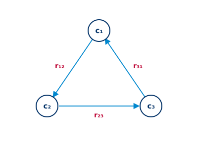
This is a gain graph: a digraph whose edges carry an invertible gain , with the reverse edge carrying . At a fixed exchange rate without fees the gain function is linear, which matters: a single series of trades (a path) always dominates any blend of trades (a flow), so we only ever need to look for a cycle. The gain of a cycle is the product of its edge gains,
and an arbitrage exists whenever some cycle has gain .
Arbitrage is a negative cycle
Taking logarithms turns the product into a sum and the search into a classic one. Weight each edge with ; then a gain above 1 is exactly a cycle of negative total weight:
Commissions slot straight in. If an exchange charges a percentage fee per transaction, the gain function is still linear, so the same reasoning applies with one extra term per edge:
Complexity
Finding a gain-generating cycle is finding the longest path from a node back to itself (or, in the log-sum form, a shortest negative one). In a complete graph the number of distinct cycles is
and a currency graph, tradable in both directions, has twice that. This grows far too fast to enumerate.
Deciding whether a graph contains a path of length at least is NP-complete. It is in NP, since summing the edges of a candidate path verifies its length. It is NP-hard by reduction from the Hamilton Path problem: an efficient longest-path algorithm would answer whether the longest path in a unit-weighted graph has length , i.e. whether a Hamilton path exists.
The same hardness rules out an exact online algorithm, one allowed a finite preparation step and then required to solve a stream of inputs in polynomial time each. If one existed, feeding it the graph one edge at a time would solve longest-path in polynomial time, contradicting the reduction. And the practical scale is unforgiving: the UN recognises 182 circulating currencies, far more than can be searched exhaustively. We need approximations, and a way to know how good they are.
The Data
To benchmark the methods we used foreign-exchange tick data from GAIN Capital. A tick is registered whenever the best bid or best ask improves on one of the observed exchanges; the smallest increment is a basis point, here . Commissions for FX are quoted in basis points and can be as low as bp (); since currencies trade in lots of 100,000, fee thresholds are easily met, so the fee is modelled as a flat percentage per trade.
Markets are presumed less efficient under uncertainty, and a proxy for uncertainty is how fast prices move: volatility, scaled over a span as . EUR/USD volatility over 2007-2013 peaks sharply in late 2008. We used two datasets accordingly: the last week of 2008 (13 currencies, maximum measured volatility) and the first week of 2012 (33 currencies). Prices are stepped through with an iterator that, for each moment , holds the most recent bid and ask for every currency up to ; the algorithms run on the iterator at every sequence number in a dataset.
Four Ways to Find the Cycle
1. Exhaustive enumeration (the reference)
To know whether an approximation found the best cycle at a moment, we need the ground truth, so we precompute all cycles by backtracking. Since the graph is not complete (not every currency trades directly against every other) and the tradable pairs stay fixed across a week, the set of valid cycles is computed once. For the 2008 graph (13 currencies) this yields 1,454 cycles; for the 2012 graph (33 currencies) it is already infeasible, with far too many simple cycles to enumerate.
2. Ant colony optimization
The first approximation borrows from nature. Ants lay pheromone on the way back from food; shorter trips refresh pheromone faster, so good routes self-reinforce. Occasionally ants get trapped reinforcing a closed loop, an ant mill, where they circle until they die of exhaustion (a behaviour reported by Schneirla). Here that pathology is the goal: we want our digital ants stuck in a gain-generating cycle.
Following Dorigo, each of ants starts at a random currency and walks the graph, using each currency at most once. The chance of moving from currency to currency blends the exchange-rate gain with the edge’s pheromone level :
When an ant returns to a currency it has already visited, a cycle is complete; its gain is added to the pheromone on each of its edges, the all-time best is saved, and after every iteration a fraction of all pheromone evaporates so that stale routes fade. The whole thing runs for iterations, giving complexity .
Does the pheromone machinery actually help? Compared against the same walk with pheromone disabled, which is to say picking random cycles, ant colony optimization averaged a gain of over 21,004 trades, versus over 18,452 for random selection. With no clear distribution over the gain cycles, the difference is not significant. Sweeping the parameters, and gave the best results for the least time.
3. Bellman-Ford
Bellman-Ford computes shortest paths from a single source by relaxation, repeatedly improving the best known distance to each vertex:
function Relax(δ, π, γ):
    for u in V:
        for v in V − {u}:
            if δ[v] > δ[u] + γ(u, v):
                δ[v] ← δ[u] + γ(u, v)
                π[v] ← u
After relaxations every acyclic shortest path from the source has been found. The detection theorem is the lever:
If after relaxations a shortest path can still be improved by one more relaxation, the graph contains a negative cycle.
The proof is short: a shortest path can hold no non-negative cycle (deleting it cannot lengthen the path), so in a graph without negative cycles all shortest paths are acyclic and at most edges long, and relaxations suffice. If a further relaxation still improves some distance to via , then a negative cycle exists and the edge lies on it. We recover the cycle by walking the predecessor pointers backwards until a node repeats. This gives a polynomial-time test for arbitrage, , with one weakness: the particular cycle returned depends on the start vertex and relaxation order.
4. Minimum mean weight cycle
The last method finds the cycle of minimum mean weight, using Karp’s characterization. The mean weight of a -edge cycle is . Add a source joined to every vertex at exchange rate 1 (weight in the log-sum form), and let be the shortest path from to using exactly edges. Then the minimum mean cycle is
We compute the table with a layered Bellman-Ford pass, store predecessors, and recover the cycle’s edges with a prefix-cost array , the cumulative cost down the retrieved path, so that checking whether a subpath of the right length realises is a constant-time lookup .
The catch is that minimum mean weight is not maximum gain. The cycle with the best per-edge average is not the cycle with the best total return.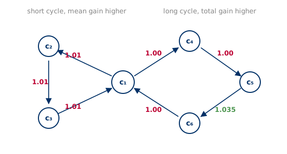
Results
Averaged over the whole 2008 dataset, Bellman-Ford is the fastest by a wide margin: it maintains two length- vectors ( and ), where the minimum mean cycle needs a full matrix.
| Method | Theoretical complexity | Time (ms) |
|---|---|---|
| Precomputed cycles | cycle number | 0.4587 |
| Bellman-Ford | $\mathrm{O}( | V |
| Minimum mean cycle | $\mathrm{O}( | V |
| Ant colony | $\mathrm{O}(I\,A\, | V |
The arbitrage opportunities themselves are small and fleeting. The best opportunity over the whole week was , a gain. Gain-generating cycles up to length 11 turn up, but the longest cycle that is ever the best at a given moment is 7.
| Method | Opportunities | Avg gain | Avg length | Longest | Best cycle |
|---|---|---|---|---|---|
| Precomputed cycles | 42,217 | 1.00076 | 3.19 | 7 | 1.006380 |
| Bellman-Ford | 42,217 | 1.00071 | 3.55 | 7 | 1.006172 |
| Minimum mean cycle | 42,018 | 1.00075 | 3.08 | 6 | 1.006380 |
| Ant colony | 15,480 | 1.00070 | 4.12 | 7 | 1.006058 |
Bellman-Ford finds an arbitrage at every one of the 42,217 moments the exhaustive reference does, confirming that if an opportunity exists in the graph, the negative-cycle test detects it. The minimum mean cycle method matches the very best cycle but visibly favours short ones, never finding a cycle longer than 6. Ant colony optimization detects far fewer opportunities and, as already noted, barely beats random search.
Discussion
If the data is correct, arbitrage opportunities do exist in foreign exchange, even after commissions. Strictly, each one means the prices are momentarily outside equilibrium, a small dent in the efficient market hypothesis. The more interesting result is the computational one: pricing all publicly available information, once “all information” includes implicit prices, is NP-hard. The law of one price can fail not because traders are irrational but because finding the mispricing is intractable in general. Good polynomial-time approximations exist, and Bellman-Ford in particular gives an exact, polynomial test for whether an arbitrage exists, even if the specific cycle it returns is arbitrary.
The caveats are real. GAIN Capital does not publish its sources, so the dataset likely covers only a slice of exchanges; latency between observer and exchange means the price seen at time may not be the price on the exchange at , and the same relativity bites when a trade is submitted and the market moves while the order travels. The natural next step is data with volume and full market depth at every price change, rather than top-of-book bid/ask alone.
A decade later. I would no longer call this a dent in the efficient market hypothesis. Opportunities this small and this short-lived, once latency and the bid-ask spread are accounted for, are roughly what a near-efficient market looks like. Efficiency is a limiting fiction, held in place by the very arbitrageurs who profit from violating it. Grossman and Stiglitz (1980) put the point sharply: a perfectly efficient market cannot exist, because then no one would be paid to gather the information that makes it efficient. My original reading, that these prices are technically outside equilibrium, I still hold. It simply points somewhere other than market efficiency. It points at markets as out-of-equilibrium systems, which is the direction my later work took.
The computational angle survives in a sharper form. The honest claim is not that markets are hard and therefore inefficient. It is that complexity creates asymmetry. Arora, Barak, Brunnermeier, and Ge (2011) show that structured products can hide junk that is NP-hard to detect, by reduction from densest subgraph, so intractability can let a seller sustain a mispricing that a buyer cannot efficiently uncover.
Takeaways
- FX arbitrage is a negative-cycle problem: weight each rate by and an arbitrage is a negative-weight cycle, commissions included.
- Searching for the best cycle is NP-hard (via Hamilton path), but detecting an arbitrage is polynomial: Bellman-Ford does it in and was both the fastest and the most reliable method tested.
- Nature-inspired search (ant colony) underwhelmed here, barely beating random cycles; Karp’s minimum mean weight cycle is elegant but optimises the wrong objective, preferring short cycles to high-gain ones.
- Arbitrage opportunities were present even net of fees: tiny () and short-lived, but real in this data.
This is the last of three problems from the dissertation. The others cast debt resolution and portfolio diversification as graph problems in the same spirit.
References
- R. M. Karp (1978). A Characterization of the Minimum Cycle Mean in a Digraph. Discrete Mathematics 23(3).
- M. Dorigo (1992). Optimization, Learning and Natural Algorithms. PhD thesis, Politecnico di Milano.
- T. C. Schneirla (1944). A unique case of circular milling in ants. American Museum Novitates.
- A. V. Goldberg and T. Radzik (1993). A heuristic improvement of the Bellman-Ford algorithm. Applied Mathematics Letters 6(3).
- R. E. Bellman (1958), L. R. Ford Jr. The shortest-path relaxation algorithm.
- S. J. Grossman and J. E. Stiglitz (1980). On the Impossibility of Informationally Efficient Markets. American Economic Review 70(3).
- S. Arora, B. Barak, M. Brunnermeier, and R. Ge (2011). Computational Complexity and Information Asymmetry in Financial Products. Communications of the ACM 54(5).